Benchmark

Reproducible build / solve / memory comparison between polar-high, linopy, and Pyomo on indexed linear programs, all using HiGHS as the solver. The dense-LP test follows linopy's benchmark, restricted to the linear case so polar-high can run it directly.

The benchmark is a manual artefact, not a CI workflow; runner variability would make CI numbers misleading. The model code, runner, and plot script live under benchmark/ so anyone can re-run on their own hardware in a few minutes.

Headline — dense LP, build-only, single-thread

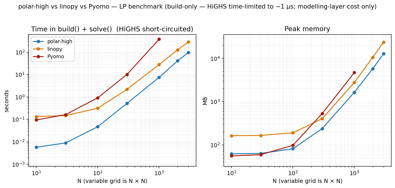
Two panels: total time = build() + solve(), and peak memory. HiGHS is time-limited to 1 µs so the column reflects pure modelling-layer cost: what each tool spends turning Python into something HiGHS can chew on. polar-high and linopy run at POLARS_MAX_THREADS=1 / OMP_NUM_THREADS=1. Pyomo is single-threaded by design.

The dense LP that drives this figure (linopy's original model, restricted to LP):

min  Σ_{i,j} (2·x[i,j] + y[i,j])
s.t. x[i,j] - y[i,j] >= i          for i,j ∈ {1,…,N}
     x[i,j] + y[i,j] >= 0          for i,j ∈ {1,…,N}
     x, y >= 0

Variables: 2·N². Constraints: 2·N². Closed-form optimum obj = N²·(N+1), used as the cross-tool correctness anchor.

At N=3000 (a 18 M-variable LP):

	total time	peak memory
polar-high	96 s	12.7 GB
linopy	290 s	23.6 GB
Pyomo	(caps at N=1000)	(4.7 GB at N=1000)

polar-high is roughly 3× faster than linopy and uses about half the memory at N=3000. Pyomo's per-coefficient Python overhead makes it unable to keep up past N≈1000 in our 10-minute timeout.

Note on the memory column

Peak RSS scales roughly linearly with nnz for all three tools, but the slope between Pyomo and the columnar tools differs by an order of magnitude. Pyomo carries each LP coefficient as a small Python expression-tree node (a VarData reference plus a numeric multiplier inside a MonomialTermExpression). CPython stores each of those at roughly 100–200 bytes once header, type pointer, refcount, and per- object dict are accounted for. polar-high and linopy hold coefficients as contiguous Arrow / numpy buffers of about 16 bytes per nonzero. At 4 M nonzeros the representation difference compounds to a multi-GB peak gap.

Between the two columnar tools the comparison flips depending on the test:

• At full HiGHS solve (the linopy-format replication figure below): linopy's peak at N = 1000 is below polar-high's. xarray's dense-broadcast representation is genuinely compact on this regular N × N grid, and HiGHS's own working set then dominates everyone's total.
• In the build-only headline above: polar-high sits below linopy at large N. Two factors contribute, in unknown proportion. First, streaming constraint assembly (polar-high emits LP rows per family and releases each family's intermediates before the next; linopy materialises all coefficients at once). Second, the LP-file vs direct handoff (the build-only test exercises linopy's io_api="lp" path, the configuration where our time_limit short-circuit reliably reaches HiGHS, which serializes the LP through an intermediate text format; polar-high skips that step via highspy).

The take-away: which tool wins on memory depends on which phase of the build/solve cycle dominates your run. Re-run on your own model before assuming any of these ratios apply.

Reproducing

git clone https://github.com/nodal-tools/polar-high.git
cd polar-high
pip install -r benchmark/requirements.txt
python benchmark/run.py            # ~10 min on a laptop
python benchmark/plot.py           # writes docs/assets/benchmark*.png

benchmark/run.py accepts --sizes, --tools, --threads, --repeats, --time-limit. Each (tool, N) cell runs in a fresh subprocess so caches and Python state don't carry over. The plot takes the median across reps. See benchmark/README.md for the methodology details.

Threading: defaults and where it matters

polar-high sets POLARS_MAX_THREADS=1 at import. The data below shows why.

Scaling with threads at small N

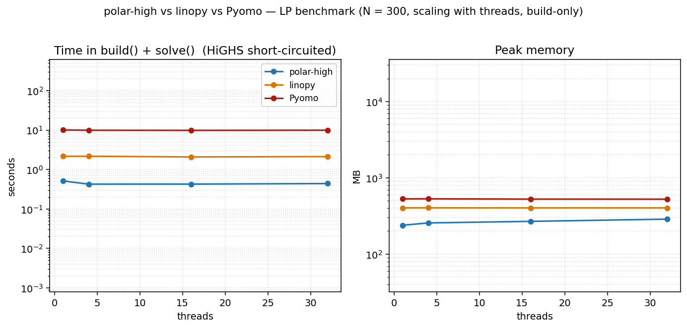
At a small problem size (N=300) the build is too small to amortize Rayon's coordination overhead. All three tools are essentially flat across thread counts. polars's parallelism doesn't pay; linopy and Pyomo are single-threaded by design. polar-high's peak memory rises slightly with threads (per-thread scratch buffers, ~1.5 MB per thread on this LP) without a corresponding time win.

Scaling with threads on a larger LP

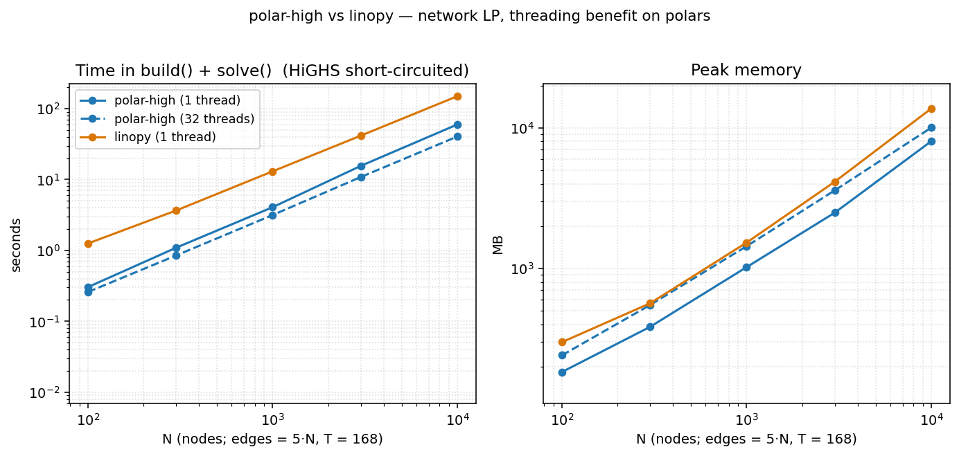
On the network LP (irregular topology, T=168, see below), polar's threading does start paying as N grows, and grows steadily:

N	polar 1 thread	polar 32 threads	speedup
100	0.30 s	0.26 s	1.16×
300	1.08 s	0.84 s	1.29×
1 000	4.08 s	3.18 s	1.28×
3 000	15.5 s	10.8 s	1.43×
10 000	60.0 s	40.5 s	1.48×

At threads=32, polar uses ~25 % more memory than at threads=1 (per-thread Rayon scratch). The takeaway:

• Default threads=1 is the right choice for typical workloads. Faster and leaner on small/medium LPs; only modestly slower than threads=32 even at large N.
• Override to threads=N by setting POLARS_MAX_THREADS before importing polar-high. Worth doing for genuinely large indexed LPs where you've checked that the polars-side build is the bottleneck.

POLARS_MAX_THREADS=8 python my_model.py

Network LP: irregular topology

The dense N × N headline above is the model linopy's benchmark uses, and it's flattering to xarray: every cell has the same shape, indexing is rectangular, and dense numpy arrays compress the coefficient matrix. Real indexed LPs (energy systems, supply chains) aren't shaped that way. They have irregular topology: flow variables on edges, balance constraints on nodes, with an edge→node lookup that varies per node.

The network LP captures that:

N nodes, E = 5·N edges drawn at random (Hamiltonian cycle + 4·N random),
T = 168 time steps (one week of hours)

vars     flow[e, t] >= 0
cstr 1   flow[e, t] <= cap[e, t]                                  ∀ (e, t)
cstr 2   Σ_{e: dst[e]=n} flow[e,t] − Σ_{e: src[e]=n} flow[e,t]
                                            == demand[n, t]       ∀ (n, t)
obj      min Σ cost[e] · flow[e, t]

The node-balance constraint requires an edge→node lookup. polar-high expresses this as a polars join (Where(flow, edges_dst_n)); linopy uses flow.groupby(dst_array).sum(); Pyomo precomputes incoming[n] adjacency dicts and iterates them. Each idiom is natural to its tool.

At N=10 000 (≈ 8.4 M variables, ≈ 10 M constraints):

	total time	peak memory
polar-high	60 s	8.0 GB
linopy	146 s	13.7 GB
Pyomo	timed out at N=3000	—

polar wins all three columns and Pyomo can't finish at this scale inside our 10-minute timeout. Notably, linopy's memory advantage on the dense LP doesn't carry over here. The irregular (e, t) → (n, t) join breaks xarray's dense-broadcast pattern, while polar's join semantics map naturally onto the operation.

Replication: linopy's original benchmark format

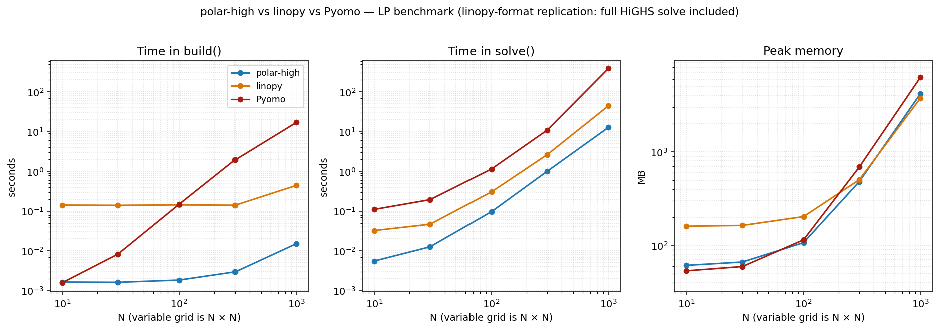
This is the same dense LP at threads=1 in the linopy benchmark's original three-panel format: build / solve / memory shown separately, with the full HiGHS solve included (no time limit). We include it for direct visual comparison with linopy's published numbers and as the methodology footnote.

Caveat: read with care. The build() / solve() split is not an apples-to-apples decomposition across tools. Each library draws the boundary in a different place:

• polar-high's build() registers metadata only. The matrix assembly happens inside solve() alongside the HiGHS call.
• linopy's build() materialises xarray coefficient arrays eagerly; solve() writes them to an LP file and hands it to HiGHS.
• Pyomo's build() instantiates VarData / ConstraintData / MonomialTermExpression Python objects per coefficient. Most of the work happens here; solve() walks the expression tree to emit the LP.

So when you compare the build column between tools, you're comparing what each tool chose to put in build(). The apples-to-apples cross-tool measurement is build() + solve(), which is the headline figure at the top of this page.

That said, the replication is faithful: the closed-form objective is hit exactly, the model is the same LP, and HiGHS solves the same sparse matrix. linopy's numbers reproduce within run-to-run noise.

Fairness caveats

• Each tool builds the LP in its own natural style; the closed-form objective (or cross-tool agreement on the network LP) confirms they're all solving the same problem.
• Pyomo's solve uses the appsi_highs persistent-solver interface, the fastest Pyomo→HiGHS path. The file-based SolverFactory("highs") route would inflate Pyomo's solve time with LP-write/reread overhead.
• linopy uses io_api="lp" explicitly: the configuration where our time_limit short-circuit reliably reaches HiGHS for the build-only test. linopy's io_api="direct" is faster on full solves but interacts awkwardly with the time-limit short-circuit.
• polar-high's solve calls into highspy directly with no intermediate file in either configuration.
• HiGHS itself stays at 1 thread across all tools, so the solve column remains apples-to-apples.
• Each (tool, N) cell runs in a fresh Python process, so caches and memory don't carry over between cells. Python startup costs ~50 ms per cell, negligible at our sizes.
• One machine, one Python version, one HiGHS version. Re-run on your own hardware before reading too much into the absolute numbers; the ratios between tools are what's portable.

What's not in the benchmark

• MIP, QP, warm starts, and Lagrangian decomposition. The benchmark deliberately exercises the matrix-assembly path on plain LPs.
• JuMP and gurobipy. Both have toolchain or licence friction that defeats "anyone can re-run from a clean pip install".

If you'd like a different model class (block-angular, time-coupled, mixed-integer with branching) in the benchmark, open an issue. The runner is a small enough surface to extend.